- Published on
Visual exploratory analysis with pydeck
- Authors
- Name
- Lorenzo Perozzi
- @lperozzi


Overview
This tutorial is part of a Data Science Tools meeting organized by the Data Science Competence Center (CDD) of the University of Geneva (Switzerland).
- About
- Setup instruction
- Import packages
- Load and inspect the dataset
- Reproject coordinate from EPSG:2056 to EPSG:4326
- Retrieve depth of geothermal probes
- Interactive visual exploration using
About
Geothermal is a hot topic right now in Switzerland and especially in the Canton of Geneva. The ongoing 3D seismic exploration campaign, which aims to better understand the subsurface structures and geological properties and develop geothermal energy that will be integrated into the district heating of the Canton of Geneva, to reduce the dependence on fossil fuels. For the moment, geothermal probes are the most common method of using geothermal heat in Switzerland. The probes extract geothermal energy from the soil and conduct it via a heat pump to a heating system.
During this tutorial, it will be shown how to use python to process and visualize a dataset about geothermal probes availability in the Canton of Geneva. This dataset can be obtained (open access) through the SITG (Système d’Information du Territoire à Genève). We will cover these aspects:
- Load the geothermal probes dataset from the Système d’Information du Territoire à Genève (SITG);
- Convert CRS coordinate system with
pyproj; - Extract depth information from attributes;
- Visualizing the results with
pydeck;
Setup instruction
If you want to follow along the tutorial, make sure you've done these steps before the tutorial begin:
Step 1
Install a Python distribution:
In this tutorial we will be using the Anaconda
Python distribution along with the conda package manager. If you already have
Anaconda or Miniconda installed, you can skip this step.
If not, please follow the instructions for getting Anaconda up and running in your system: https://docs.anaconda.com/anaconda/install/
Step 2
Create the DST-geothermal-visual conda environment:
- Clone this repository;
- Open a terminal (Anaconda Prompt if you are running Windows). The following steps should be done in the terminal;
- Navigate to the folder that has been cloned (if you don't know how to do this, take a moment to read the Software Carpentry lesson on the Unix shell);
- Create the conda environment by running
conda create -n DST-geothermal-visual(this will download and install all of the packages used in the tutorial); - Windows users: Make sure you set a default browser that is not Internet Explorer;
- Installing
pipin the new environment:conda install -n DST-geothermal-visual pip; - Activate the conda environment:
conda activate DST-geothermal-visual; - Installing packages to run the tutorial:
pip install ipython pandas numpy matplotlib pyproj pydeck jupyterlab; - Create a new kernel for this environment environment:
ipython kernel install --user --name=DST-geothermal-visual; - Start the JupyterLab server:
jupyter lab; - Open the
Visual analyisis of geothermal probes with pydeck.ipynbto follow the tutorial or a new fresh Notebook if you want to start form scratch. Be sure the kernel is set toDST-geothermal-visual; - Feel free to open an issue if you have some problem during the installation or during the tutorial.
Import packages
import pydeck
import pandas as pd
import numpy as np
import matplotlib.cm
import matplotlib.pyplot as plt
import warnings
warnings.filterwarnings('ignore')  # filter out warning messages

plt.rcParams['figure.dpi'] = 150 # plot bigger figure inline
Load and inspect the dataset
The dataset is stored on the SITG (Système d'information du territoire à Genève) and publicly available.
filename = 'data/CTSS_CHAUFFAGE_SONDE.csv'
To open the dataset we use the Pandas package. By default in a csv file, columns are separated by a comma (,), however, we can specify different methods for this. In this tutorial, the dataset columns are separated by a semicolon, we need then to specify the sep arguments in the pd.read_csv class.
sondes = pd.read_csv(filename, encoding='latin-1', sep=';')
We can inspect the dataset.
sondes.head(5) # first 5 rows
====  ==========  ============  ==============  ==============  ==================================  ====================  ==========  =============================  =========================  ===========  ===========
  ..    ID_SONDE  ID_DOSSIER      ALTITUDE_MIN    ALTITUDE_MAX  DIMENSION                           FLUIDE                ETAT        DETERMINATION_PLANIMETRIQUE    REMARQUES                            E            N
====  ==========  ============  ==============  ==============  ==================================  ====================  ==========  =============================  =========================  ===========  ===========
   0         nan  APA 29428                  0               0  Diamètre 32mm/40mm Profondeur 130m  Glycol / Alcoll 30 %  En service  Précis                         Selon plan d'implantation  2.50313e+06  1.11669e+06
   1         nan  DD103532                   0               0  Profondeur 150m                     Inconnu               En service  Précis                         Selon plan d'implantation  2.50397e+06  1.11748e+06
   2         nan  DD103532                   0               0  Profondeur 150m                     Inconnu               En service  Précis                         Selon plan d'implantation  2.50397e+06  1.11748e+06
   3         nan  DD 103116                  0               0  Diamètre 32mm Profondeur 126m       Inconnu               En service  Précis                         nan                        2.50038e+06  1.12468e+06
   4         nan  DD 103116                  0               0  Diamètre 32mm Profondeur 126m       Inconnu               En service  Précis                         nan                        2.50039e+06  1.12469e+06
====  ==========  ============  ==============  ==============  ==================================  ====================  ==========  =============================  =========================  ===========  ===========
By using the .info() methods we can retrieve more details about the dataset such as the total number of rows and columns, the type of the columns, and so on.
sondes.info()
<class 'pandas.core.frame.DataFrame'>
RangeIndex: 2033 entries, 0 to 2032
Data columns (total 11 columns):
 #   Column                       Non-Null Count  Dtype
---  ------                       --------------  -----
 0   ID_SONDE                     170 non-null    object
 1   ID_DOSSIER                   1933 non-null   object
 2   ALTITUDE_MIN                 1888 non-null   float64
 3   ALTITUDE_MAX                 1965 non-null   float64
 4   DIMENSION                    1548 non-null   object
 5   FLUIDE                       2031 non-null   object
 6   ETAT                         1989 non-null   object
 7   DETERMINATION_PLANIMETRIQUE  1982 non-null   object
 8   REMARQUES                    481 non-null    object
 9   E                            2033 non-null   float64
 10  N                            2033 non-null   float64
dtypes: float64(4), object(7)
memory usage: 174.8+ KB
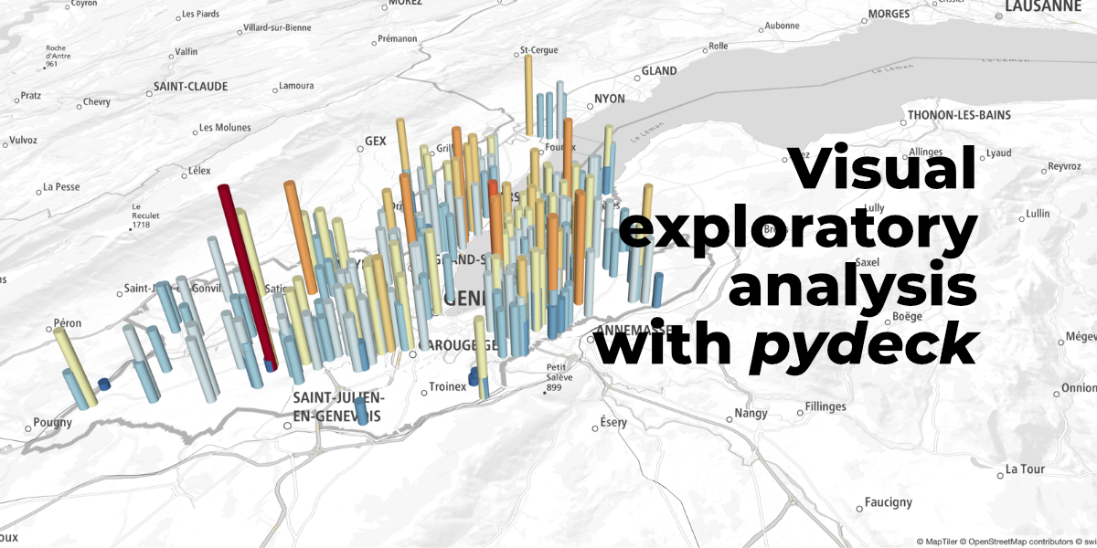
The file contains 11 columns (attributes) and 2033 entries. The objective here is to analyse/visualize the geothermal probes using pydeck, an high-scale spatial rendering powered by deck.gl. We need at least 3 attributes: the spatial coordinates (X and Y) as well as the depth of each probes.
In the dataset the only attributes that do not have NaN values are E and N corresponding to the Easting and Northing coordinates.
sondes[['E','N']].head(5)
====  ===========  ===========
  ..            E            N
====  ===========  ===========
   0  2.50313e+06  1.11669e+06
   1  2.50397e+06  1.11748e+06
   2  2.50397e+06  1.11748e+06
   3  2.50038e+06  1.12468e+06
   4  2.50039e+06  1.12469e+06
====  ===========  ===========
E and N are in the CH1903+_LV95 reference system (also known as EPSG:2056).
To visualize the data with pydeck (and in general with all geospatial visualization packages) however, we need to work on World Geodetic System 1984 - WGS84 (also know as EPSG:4326).
The first step will then reproject the data from the EPSG:2056 system to the EPSG:4326 system.
Reproject coordinate from EPSG:2056 to EPSG:4326
There are several online converters for that such as EPSG.io, which works well when we have a few sets of coordinates to transform. However, to be efficient, we use pyproj that is a Python interface to PROJ (cartographic projections and coordinate transformation library).
from pyproj import Transformer
from pyproj import CRS
- Initializing CRS and creating a transformer to convert from 2056 to 4326.
crs_4326 = CRS.from_epsg(4326)
crs_2056 = CRS.from_epsg(2056)
transformer = Transformer.from_crs(crs_2056, crs_4326)
- Convert
EandNtoLatitudeandLongituderespectively.
sondes['lat'], sondes['lon'] = transformer.transform(sondes.E.values, sondes.N.values)
sondes[['E','N','lat','lon']].head(5)
====  ===========  ===========  =======  =======
  ..            E            N      lat      lon
====  ===========  ===========  =======  =======
   0  2.50313e+06  1.11669e+06  46.1947  6.18383
   1  2.50397e+06  1.11748e+06  46.2019  6.19449
   2  2.50397e+06  1.11748e+06  46.2019  6.19454
   3  2.50038e+06  1.12468e+06  46.2661  6.14651
   4  2.50039e+06  1.12469e+06  46.2662  6.14663
====  ===========  ===========  =======  =======
Retrieve depth of geothermal probes
We want also know the depth of the geothermal probes. In the dataset we do not have an attribute for that, we need further inspection. Among the 11 columns we have ALTITUDE_MIN, ALTITUDE_MAX and DIMENSION that should give us this information. However, these attributes contain several NaN. Let's inspect these attributes.
sondes[['ALTITUDE_MIN','ALTITUDE_MAX','DIMENSION']].sample(8, random_state=51)
====  ==============  ==============  ===============================
  ..    ALTITUDE_MIN    ALTITUDE_MAX  DIMENSION
====  ==============  ==============  ===============================
1024               0           374    Diamètre 4x32mm Profondeur 137m
1255               0           393.8  Diamètre 40mm Profondeur 185m
 907               0             0    diamètre 32mm profondeur 290m
1763               0             0    nan
1181               0           455.5  4x diamètre 32mm Profondeur 85m
1136             nan           451.3  Diamètre 4x32mm Profondeur 140m
  18               0             0    Profondeur 90m
1301               0             0    nan
====  ==============  ==============  ===============================
We have several cases:
NaNeverywhere, we will drop these lines while useless- Depth information contained in the
DIMENSIONattributes, as a string text - Depth information contained in the (
ALTITUDE_MAX-ALTITUDE_MIN) attributes, as a string text
Note: Normally, with pd.read_csv() the NaNs are automatically detected, however, depending on how the data have been compiled, it is not always the case. For example, the 0.0 value in ALTITUDE_MAX or ALTITUDE_MIN attribute corresponds clearly to NaNs values.
The next step will be to clean up all lines that contain NaN.
sondes.replace(to_replace=0.0, value=np.NaN, inplace=True)
sondes[['ALTITUDE_MIN','ALTITUDE_MAX','DIMENSION']].sample(8, random_state=51)
====  ==============  ==============  ===============================
  ..    ALTITUDE_MIN    ALTITUDE_MAX  DIMENSION
====  ==============  ==============  ===============================
1024             nan           374    Diamètre 4x32mm Profondeur 137m
1255             nan           393.8  Diamètre 40mm Profondeur 185m
 907             nan           nan    diamètre 32mm profondeur 290m
1763             nan           nan    nan
1181             nan           455.5  4x diamètre 32mm Profondeur 85m
1136             nan           451.3  Diamètre 4x32mm Profondeur 140m
  18             nan           nan    Profondeur 90m
1301             nan           nan    nan
====  ==============  ==============  ===============================
Then we remove all rows with NaN in ALTITUDE_MAX, ALTITUDE_MIN, DIMENSION
sondes.dropna(subset=['ALTITUDE_MIN', 'ALTITUDE_MAX', 'DIMENSION'], thresh=2, inplace=True)
sondes[['ALTITUDE_MIN','ALTITUDE_MAX','DIMENSION']].sample(8, random_state=51)
====  ==============  ==============  ==========================================
  ..    ALTITUDE_MIN    ALTITUDE_MAX  DIMENSION
====  ==============  ==============  ==========================================
 390          233.11          393.11  Long.max.160ml,4 sondes diam.34mm par tube
 948          134             404     nan
1485          300             433     nan
 861          nan             395.5   Diamètre 4x40mm Profondeur 135m
1080          nan             434.7   Profondeur 135m
 373          303.8           428.8   Long. totale = 125ml / Diam. 4 x 32
 822          nan             383     Diamètre 4x32mm Profondeur 150m
1129          nan             433.9   Diamètre 4x 32mm Profondeur 160m
====  ==============  ==============  ==========================================
We then need to create a DEPTH attributes that retrieve geothermal probe information from ALTITUDE_MIN and ALTITUDE_MAX, if these attributes do not contain NaN...
sondes.reset_index(inplace=True)
idx1 = np.where((~np.isnan(sondes['ALTITUDE_MIN'].values)) & (~np.isnan(sondes['ALTITUDE_MAX'].values)))
sondes['DEPTH'] = np.nan
sondes['DEPTH'].loc[idx1] = sondes.ALTITUDE_MAX - sondes.ALTITUDE_MIN
sondes[['ALTITUDE_MIN','ALTITUDE_MAX','DIMENSION', 'DEPTH']].sample(8, random_state=2)
====  ==============  ==============  ===============================  =======
  ..    ALTITUDE_MIN    ALTITUDE_MAX  DIMENSION                          DEPTH
====  ==============  ==============  ===============================  =======
 550             nan           400    diamètre 4x40mm Profondeur 200m      nan
 792             nan           384.1  Diamètre 4x40mm Profondeur 180m      nan
 682             nan           460    Diamètre 32mm Profondeur 120m        nan
1221             nan           453.6  Profondeur 85m                       nan
 169             222           422    nan                                  200
1212             228           428    Prof.220m.                           200
 181             273           433    nan                                  160
 481             nan           395.5  Diamètre 4x32mm Profondeur 130m      nan
====  ==============  ==============  ===============================  =======
... or from the DIMENSION column. This attribute is a string, from which we need to extract depth information. For this, we use the following regular expression str.extract('(\d+)') that allows extracting the digits from the last 5 characters of the DIMENSION string text.
idx2 = np.where((np.isnan(sondes['DEPTH'].values)))
sondes['DEPTH'].loc[idx2] = sondes['DIMENSION'].loc[idx2].str[-5:].str.extract('(\d+)', expand=False).astype(np.float32)
sondes[['ALTITUDE_MIN','ALTITUDE_MAX','DIMENSION', 'DEPTH']].sample(8, random_state=2)
====  ==============  ==============  ===============================  =======
  ..    ALTITUDE_MIN    ALTITUDE_MAX  DIMENSION                          DEPTH
====  ==============  ==============  ===============================  =======
 550             nan           400    diamètre 4x40mm Profondeur 200m      200
 792             nan           384.1  Diamètre 4x40mm Profondeur 180m      180
 682             nan           460    Diamètre 32mm Profondeur 120m        120
1221             nan           453.6  Profondeur 85m                        85
 169             222           422    nan                                  200
1212             228           428    Prof.220m.                           200
 181             273           433    nan                                  160
 481             nan           395.5  Diamètre 4x32mm Profondeur 130m      130
====  ==============  ==============  ===============================  =======
Now we have all the information needed to visualize the geothermal probes dataset with pydeck.
Interactive visual exploration using pydeck
The "Layer" is a core concept of deck.gl. A deck.gl layer is a packaged visualization type that takes a collection of datums, associate each with positions, colors, extrusions, etc., and renders them on a map. For this visualization, we use a ColumnnLayer. Read this for a deck.gl layer catalog overview.
layer = pydeck.Layer(
    'ColumnLayer',  # `type` positional argument is here
    data=sondes,
    get_position=['lon', 'lat'],
    auto_highlight=True,
    get_elevation='DEPTH',
    elevation_scale=25,
    radius=50,
    pickable=True,
    get_fill_color = [69,162,128,255],
    coverage=2)

view_state = pydeck.ViewState(
    longitude=6.183829,
    latitude=46.194656,
    zoom=10,
    min_zoom=5,
    max_zoom=15,
    pitch=25,
    bearing=0)

# Combined all of it and render a viewport
r = pydeck.Deck(layers=[layer],
                height=1500,
                initial_view_state=view_state,
               )
r.to_html('geothermal-probes-viz-1.html',open_browser=False, iframe_height=750)
The resulting visualization is a .html file that can be opened in any browser (click here to show the results in a browser)
Data and code to reproduce this work can be found here.