- Published on
Let us grab a beer in Lausanne
- Authors
- Name
- Lorenzo Perozzi
- @lperozzi


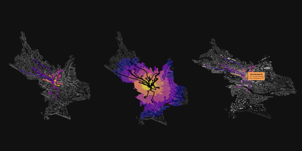
Overview
This short tutorial provide a quick tour on how download all the bars tagged as microbrewery in Lausanne from the OpenStreetMap dataset and to model the shortest path from a given point in Lausanne, Lausanne Flon to the microbrewery closest.
- Downloading the street network
- Plotting the street network
- Define the origin point
- Search for the microbrewery in Lausanne
- Shortest path
- Building footprints
- Isochrones from origin point
- Plot the time-distances as isochrones
- Additional resources
- References
Downloading the street network
OSMNx allow to download a street network from a city name (using Nominatim API), from an address, from a point (with some distance to it) or from a polygon. Here we use a polygon that include the city center of the Lausanne.
# Read a polygon extracted form QGIS as a geojson
# Get polygon boundary related to the polygon name as a geodataframe
lausanne_city_center = gpd.read_file('data/Lausanne_city_center.geojson')

# assign a shapely geometry to the polygon
lausanne_city_center_pol = lausanne_city_center.loc[0, 'geometry']
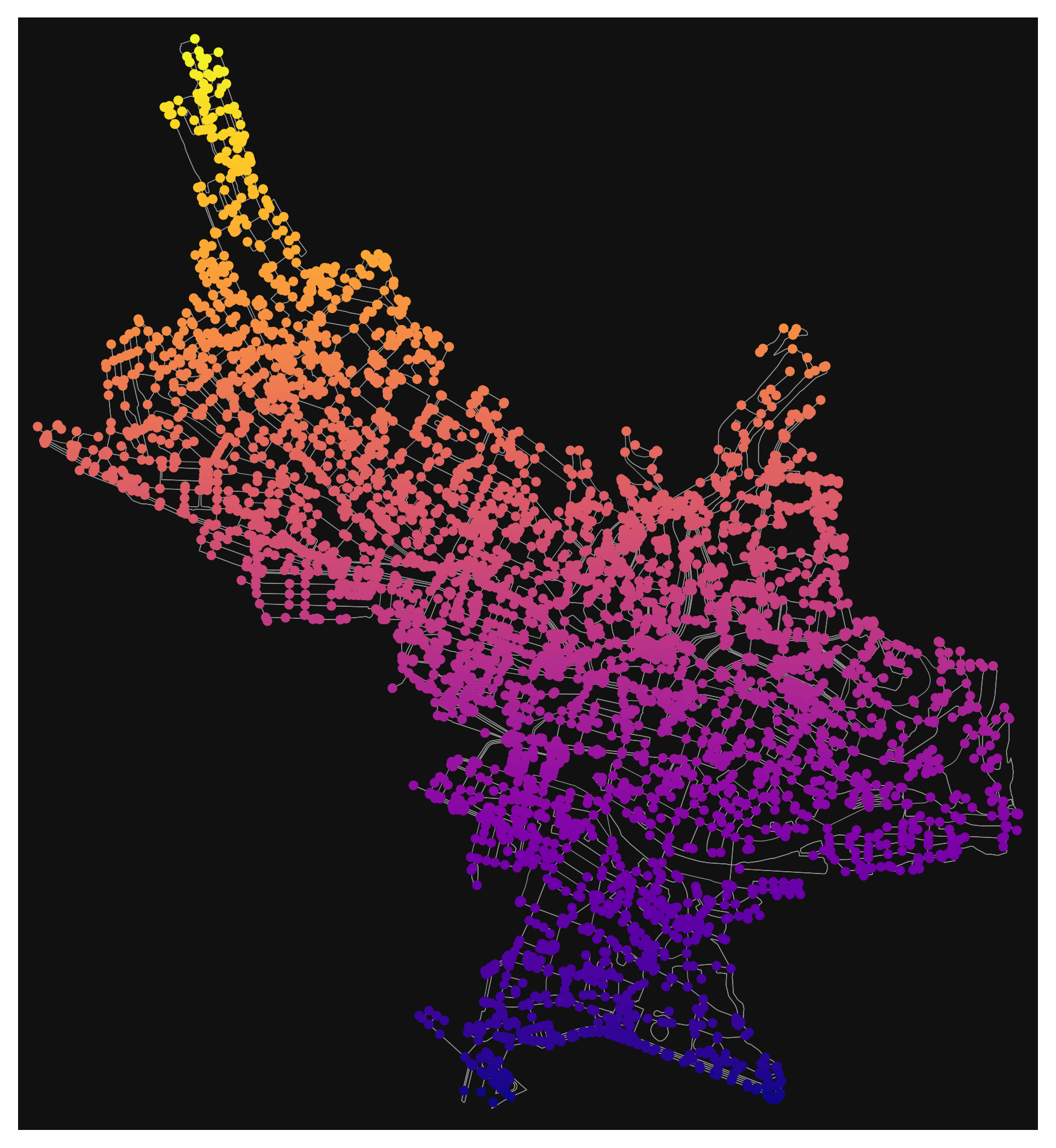
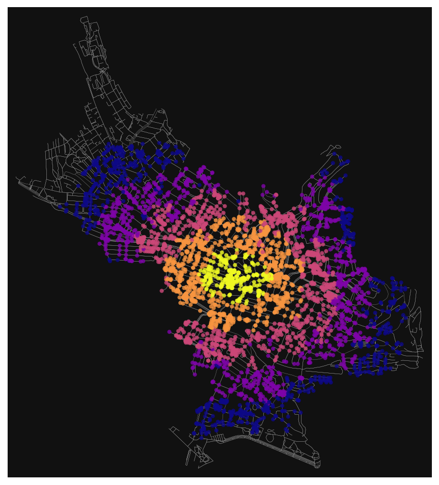
Plotting the street network
OSMnx has several plotting option. For example we can plot the network and pass an attribute to a colormap:
# Fetch OSM street network from the polygon
graph = ox.graph_from_polygon(lausanne_city_center_pol)
# get node colors by linearly mapping an attribute's values to a colormap
nc = ox.plot.get_node_colors_by_attr(graph, attr="y", cmap="plasma")
fig, ax = ox.plot_graph(graph, node_color=nc, edge_linewidth=0.3)
Define the origin point
Then we retrieve the origin point form where we want to model the shortest path to each microbrewery.
# creating the origin from Lausanne Flon
origin = gpd.GeoDataFrame(columns = ['name', 'geometry'], crs = 4326, geometry = 'geometry')
origin.at[0, 'geometry'] = Point(6.631004310693691, 46.52025924145879)
origin.at[0, 'name'] = 'Lausanne Flon'
Search for the microbrewery in Lausanne
The next step is to retrieve all the pub in Lausanne that have a tag microbrewery:yes. The microbrewery tag can be used for pubs, restaurants, etc. to indicate that there is a microbrewery on the premises
# List key-value pairs for tags
tags = {'amenity': 'pub', 'microbrewery':'yes'}
# Get the data
microbrasseries = ox.geometries_from_polygon(lausanne_city_center_pol, tags)
microbrasseries.reset_index(inplace=True)
microbrasseries.head()

microbrasseries = microbrasseries[['osmid','name', 'addr:housenumber', 'addr:street','geometry']]
microbrasseries = microbrasseries.reset_index(drop=True)
# getting centroids from polygons to avoid polygon geometric objects
microbrasseries['geometry'] = [geom.centroid for geom in microbrasseries['geometry']]
microbrasseries.head(5)
osmid	name	addr:housenumber	addr:street	geometry
0	365937679	Les Brasseurs	4	Rue Centrale	POINT (6.63258 46.52060)
1	417706015	Le XIIIe siecle	NaN	NaN	POINT (6.63530 46.52341)
2	603714714	Le Central	5	Rue Centrale	POINT (6.63203 46.52076)
3	603722682	King Size pub	16	Rue du Port-Franc	POINT (6.62694 46.52190)
4	826027336	Le Lapin Vert	2	Ruelle du Lapin Vert	POINT (6.63590 46.52359)
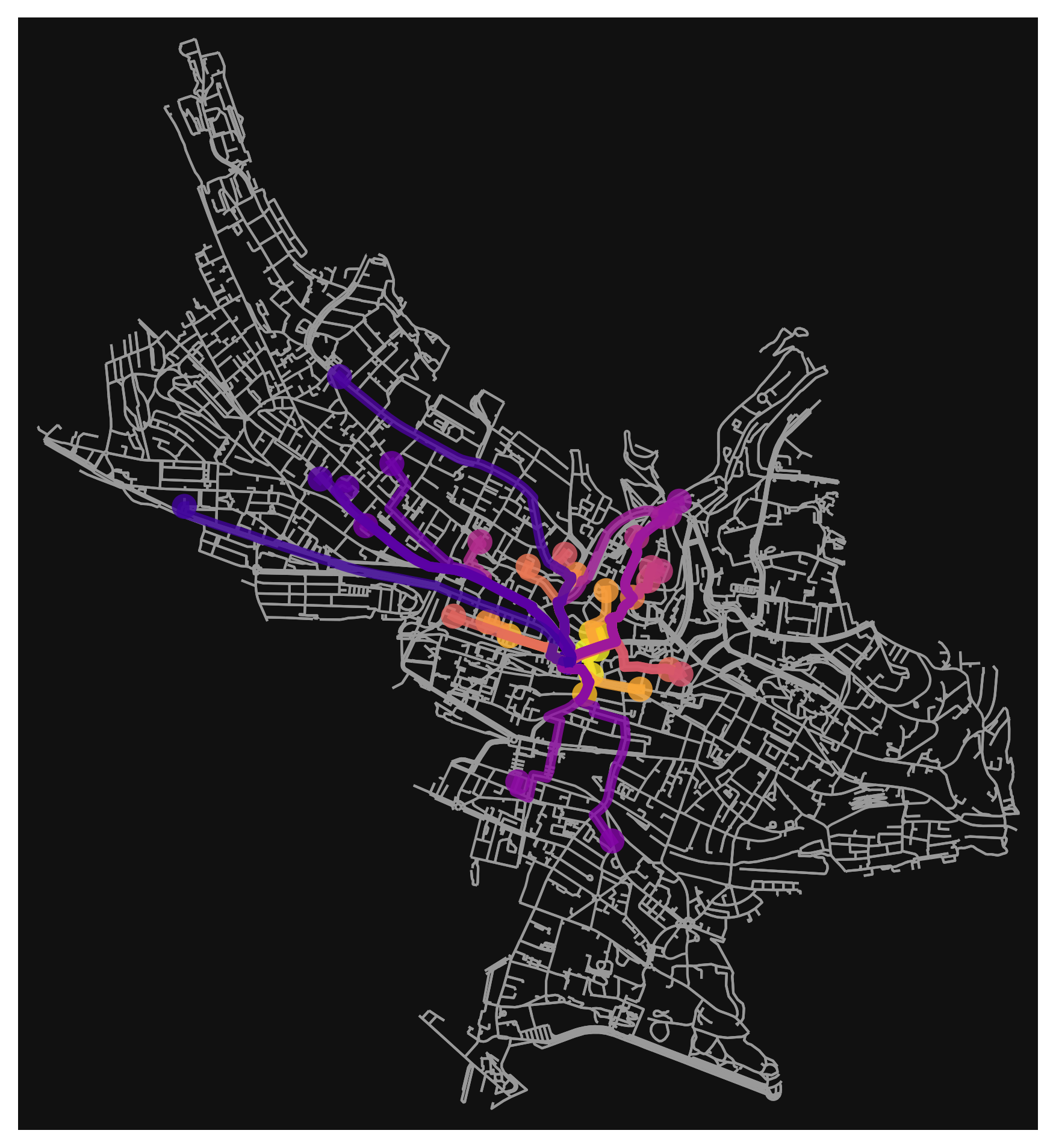
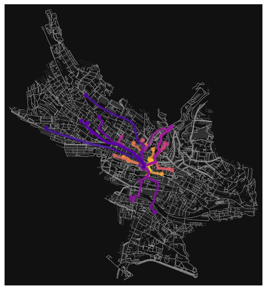
Shortest path
Now we can model the shortest path between the origin point (Lausanne Flon) and each microbrewery using the shortest path function in OSMnx
# converting the graph projection in local UTM projection
graph_proj = ox.project_graph(graph)

# get the closest node to the origin point
origin_node = ox.distance.nearest_nodes(G=graph, X=origin.geometry.x, Y=origin.geometry.y)

# get the destinations nodes (microbrewery)
destination_nodes = ox.distance.nearest_nodes(G=graph, X=microbrasseries.geometry.x, Y=microbrasseries.geometry.y)

# Get nodes from the graph
nodes = ox.graph_to_gdfs(graph_proj, edges=False)


# compute the path between origin and each microbrewery node.
routes = gpd.GeoDataFrame()
routes2 = []
route_lengths = []
for o, d in product(origin_node, destination_nodes):
    route = ox.shortest_path(graph, o, d, weight='length')
    routes2.append(route)
    # Extract the nodes of the route
    # print(route)
    route_nodes = nodes.loc[route]

    # Create a LineString out of the route
    path = LineString(list(route_nodes.geometry.values))
    # Append the result into the GeoDataFrame
    routes = routes.append([[path]])
    route_length = ox.utils_graph.get_route_edge_attributes(graph, route, "length")
    # routes.append(route)
    route_lengths.append(route_length)


# Add a column name geometry
routes.columns = ['geometry']

# Set geometry
routes = routes.set_geometry('geometry')
# set the same crs as the nodes (UTM)
routes.crs = nodes.crs

route_lengths_total = []
for l in route_lengths:
    total = sum(l)
    route_lengths_total.append(total)
and plotting the result:
# create a dataframe for plotting and exporting
df = pd.DataFrame({"route":routes2, "node_length":route_lengths, "total_length":route_lengths_total})

# plotting parameters
df_to_plot = df.sort_values(by='total_length')
rc= ox.plot.get_colors(n=len(route_lengths_total), cmap="plasma_r", stop=0.9, return_hex=True)
df_to_plot['color'] = rc
routes['color'] = rc

# plot the result
fig, ax = ox.plot_graph_routes(graph, routes=df.sort_values(by='total_length').route.values.tolist(), route_colors=rc, route_linewidth=6, route_alpha=0.8,node_size=0)
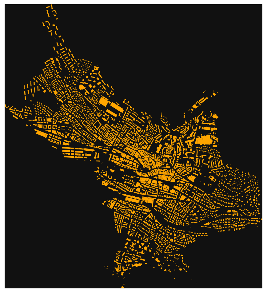
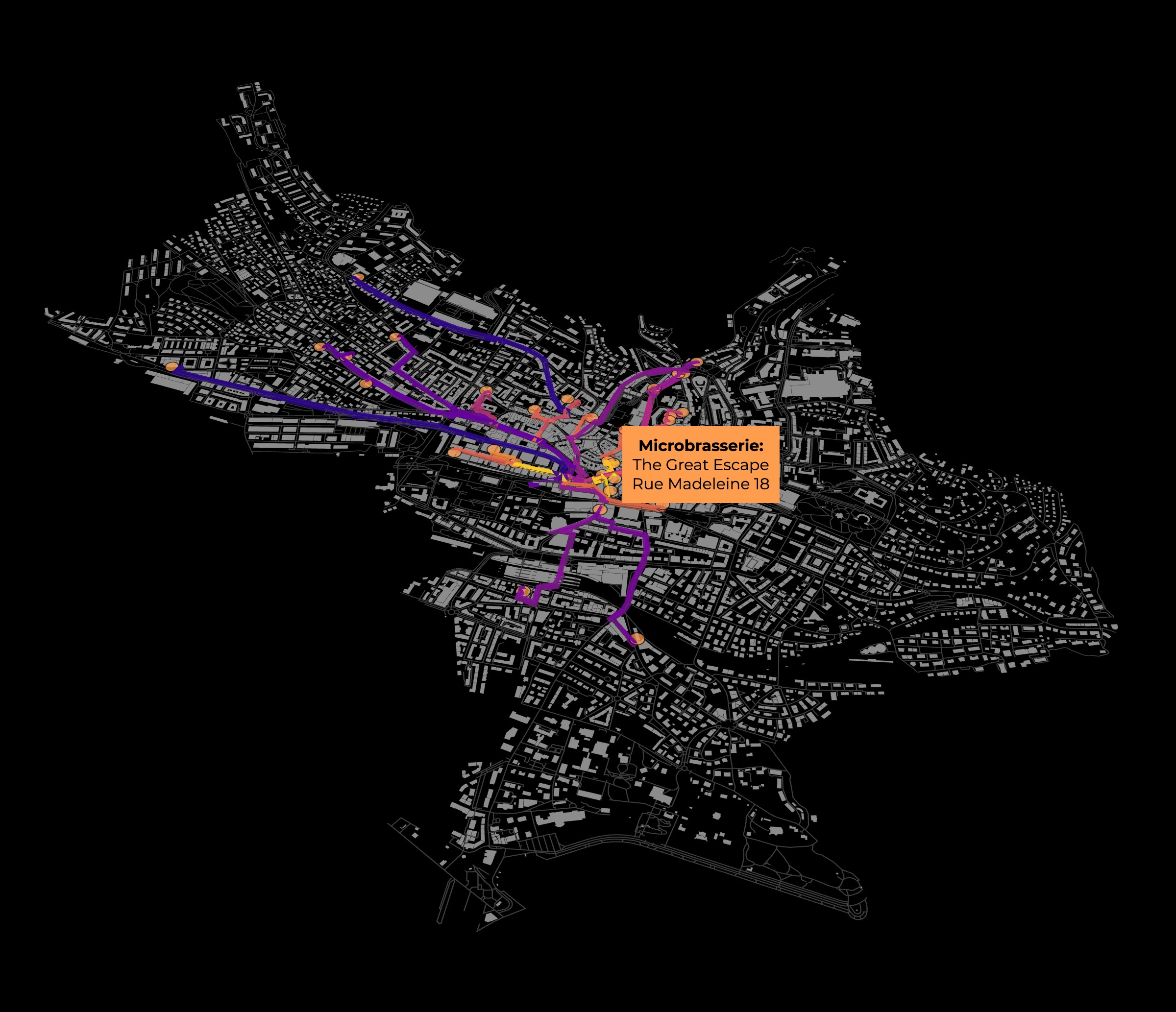
Building footprints
For improve the final visualization it is also possible to easily plot the buildings of the same areas.
# specify that we're retrieving building footprint geometries
tags = {"building": True}
gdf = ox.geometries_from_polygon(lausanne_city_center_pol, tags)
gdf_proj = ox.project_gdf(gdf)
fig, ax = ox.plot_footprints(gdf_proj, filepath=None, dpi=400, save=False, show=True, close=False)
Plotting all together gives:
fig, ax = ox.plot_footprints(gdf,alpha=0.4, color='#666666',show=False)
fig, ax = ox.plot_graph(graph, ax=ax, node_size=0, edge_color="#999999", edge_linewidth=0.5, show=False)
fig, ax = ox.plot_graph_routes(graph, ax=ax, routes=df.sort_values(by='total_length').route.values.tolist(), route_colors=rc, route_linewidth=2, orig_dest_size=50, route_alpha=0.7,node_size=0,)
This visualization is really nice, but does;nt give any information about the walking times to the brewery. What about to compute isochrones of 5, 10, 15, 20, 25 minutes from Lausanne Flon and see how far are the microbrewery?
Isochrones from origin point
We set a walking speed of 4.5 km/h that is an average speed for a gentle walk.
# add an edge attribute for time in minutes required to traverse each edge

travel_speed = 4.5 # 4.5 km/h walking speed
trip_times = [5, 10, 15, 20, 25]  # in minutes

meters_per_minute = travel_speed * 1000 / 60  # km per hour to m per minute
for _, _, _, data in graph_proj.edges(data=True, keys=True):
    data["time"] = data["length"] / meters_per_minute
we set the center node form where compute the distances
center_node = ox.distance.nearest_nodes(G=graph, X=origin.geometry.x[0], Y=origin.geometry.y[0])
we then can plot the network nodes that are reachable within the defined walking times
iso_colors = ox.plot.get_colors(n=len(trip_times), cmap="plasma", start=0, return_hex=True)

# color the nodes according to isochrone then plot the street network
node_colors = {}
for trip_time, color in zip(sorted(trip_times, reverse=True), iso_colors):
    subgraph = nx.ego_graph(graph_proj, center_node, radius=trip_time, distance="time")
    for node in subgraph.nodes():
        node_colors[node] = color
nc = [node_colors[node] if node in node_colors else "none" for node in graph_proj.nodes()]
ns = [15 if node in node_colors else 0 for node in graph_proj.nodes()]
fig, ax = ox.plot_graph(
    graph_proj,
    node_color=nc,
    node_size=ns,
    node_alpha=0.8,
    edge_linewidth=0.2,
    edge_color="#999999",
)
Plot the time-distances as isochrones
How far can you walk in 5, 10, 15, 20, and 25 minutes from the origin node? We'll use a convex hull, which isn't perfectly accurate. A concave hull would be better, but shapely doesn't offer that.
def make_iso_polys(G, edge_buff=25, node_buff=50, infill=False):
    isochrone_polys = []
    for trip_time in sorted(trip_times, reverse=True):
        subgraph = nx.ego_graph(G, center_node, radius=trip_time, distance="time")

        node_points = [Point((data["x"], data["y"])) for node, data in subgraph.nodes(data=True)]
        nodes_gdf = gpd.GeoDataFrame({"id": list(subgraph.nodes)}, geometry=node_points)
        nodes_gdf = nodes_gdf.set_index("id")

        edge_lines = []
        for n_fr, n_to in subgraph.edges():
            f = nodes_gdf.loc[n_fr].geometry
            t = nodes_gdf.loc[n_to].geometry
            edge_lookup = G.get_edge_data(n_fr, n_to)[0].get("geometry", LineString([f, t]))
            edge_lines.append(edge_lookup)

        n = nodes_gdf.buffer(node_buff).geometry
        e = gpd.GeoSeries(edge_lines).buffer(edge_buff).geometry
        all_gs = list(n) + list(e)
        new_iso = gpd.GeoSeries(all_gs).unary_union

        # try to fill in surrounded areas so shapes will appear solid and
        # blocks without white space inside them
        if infill:
            new_iso = Polygon(new_iso.exterior)
        isochrone_polys.append(new_iso)
    return isochrone_polys


isochrone_polys = make_iso_polys(graph_proj, edge_buff=25, node_buff=0, infill=True)
fig, ax = ox.plot_footprints(gdf_proj,alpha=0.4, color='#666666',show=False)
fig, ax = ox.plot_graph(
    graph_proj, ax=ax, show=False, close=False, edge_color="#999999", edge_alpha=0.2, node_size=0
)
fig, ax = ox.plot_graph_routes(graph_proj, ax=ax, show=False, routes=df.sort_values(by='total_length').route.values.tolist(), route_colors='k', route_linewidth=2, orig_dest_size=50, route_alpha=0.7,node_size=0,)

for polygon, fc in zip(isochrone_polys, iso_colors):
    patch = PolygonPatch(polygon, fc=fc, ec="none", alpha=0.7, zorder=-1)
    ax.add_patch(patch)
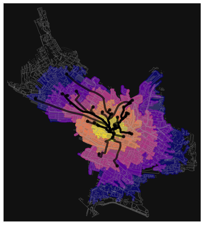
All the microbrewery are at most 25 minutes far from the Lausanne Flon, considering a gentle walk speed of 4.5 km/h. It is worth to explore them once, some of them brew really good beers.🍺🍺🍺🍺🍺
🚀🚀 If your are curious to explore interactively the microbrewery and the path to reach them from Lausanne Flon, you could download this file and open it with the browser of your choice. It should give something like this: 🚀🚀
That's it, enjoy OpenStreetMap network analysis with OSMnx, geopandas and pydeck interpolating with your own data! If you found this tutorial useful, please leave a comment below. 👇👇👇
Additional resources
There is a GitHub repository associated with this tutorial if you are interested.
There are lots of tutorials and resources on OSMnx, especially the tutorials notebook at:
References
Boeing, G. 2017. OSMnx: New Methods for Acquiring, Constructing, Analyzing, and Visualizing Complex Street Networks. Computers, Environment and Urban Systems, 65, 126-139. https://doi.org/10.1016/j.compenvurbsys.2017.05.004