Exploring spatial interpolation

Overview

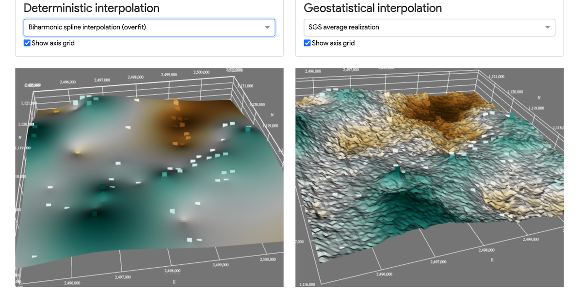
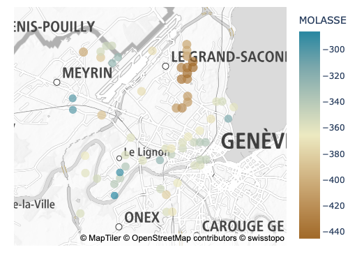
In the previous post I explained how to create a GIS webapp using plotly Dash, a productive Python framework for building web analytic applications. With this post I would like to show how we can use dash to render 3D data, using dash-vtk. With dash-vtk you can for example render a mesh representing a LiDAR dataset or a Terrain following mesh. The objective here is to compare different algorithms used to interpolate the depth of a geological unit (Molasse) in the Geneva (Switzerland) area.

There is a GitHub repository associated with this tutorial with the notebook for the spatial analysis.

The app is hosted on GitHub here and deployed on Heroku at this address https://spatial-interpolation.herokuapp.com/. Be patient, it takes a few seconds to wake app the Heroku dynos 🤞🤞.

• About
• Dataset
• Interpolation algorithms
• Nearest neighbors
• Biharmonic spline (default)
• Biharmonic spline (cross validated)
• Gaussian Processes
• Kriging
• Sequential Gaussian Simulation
• Additional resources
• Data analytics
• Web app
• Python packages

About

The dataset used in this tutorials is from the well land register managed by the geological survey of the Canton of Geneva (GESDEC) and it is part of the open data catalogue of the SITG (Système d’Information du Territoire à Genève). It can be downloaded here. from this dataset we want to interpolate the depth of the Molasse over a subregion of the Geneva, using the following interpolation algorithms:

• Nearest-neighbors;
• Biharmonic spline (using Verde);
• Gaussian processes;
• Kriging;
• Sequential Gaussian Simulation;

Dataset

The dataset can be downloaded here or fetched using the opendata.swiss API as follows:

from zipfile import ZipFile
import urllib.request
from io import BytesIO
data_url = 'https://ge.ch/sitg/geodata/SITG/OPENDATA/4108/CSV_GOL_SONDAGE.zip'


zip_file = ZipFile(BytesIO(urllib.request.urlopen(data_url).read()))

dfs = {text_file.filename: pd.read_csv(zip_file.open(text_file.filename),           encoding='ISO-8859-1', 
sep=';',)
       for text_file in zip_file.infolist()
       if text_file.filename.endswith('.csv')}

sondage = dfs['GOL_SONDAGE.csv']

Interpolation algorithms

Refers to these notebooks for a detailed explanation of the spatial analysis presented in the next section.

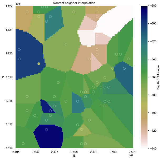
Nearest neighbors

The easiest way to apply the NN algorithm is by using the Verde package (Uieda L., 2018)¹. The dataset has been BlockReduced to a regular grid of 50m x 50m.

import verde as vd
chain = vd.Chain(
    [
        ("mean", vd.BlockReduce(np.mean, spacing=spacing )),
        ("spline", vd.ScipyGridder(method="nearest")),
    ]
)

train, test = vd.train_test_split(
    coordinates,df.MOLASSE, random_state=0
)

chain.fit(*train)

grid = chain.grid(
    region=region,
    spacing=spacing,
    dims=["N", "E"],
    data_names="MOLASSE",
)

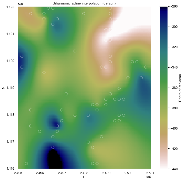
Biharmonic spline (default)

Next a biharmonic spline interpolation using Green's functions has been tested, where the two main parameters are mindist, the minimum distance the point forces and data points and damping, that controls how much smoothness is imposed on the estimated forces.

chain = vd.Chain(
    [
        ("mean", vd.BlockReduce(np.mean, spacing=spacing )),
        ("spline", vd.Spline()),
    ]
)

chain.fit(coordinates, df.MOLASSE)

grid = chain.grid(
    region=region,
    spacing=spacing,
    # projection=projection,
    dims=["N", "E"],
    data_names="MOLASSE",
)

Biharmonic spline (cross validated)

The verde.SplineCV class provides a cross-validated version of verde.Spline. It has almost the same interface but does all of the above automatically when fitting a dataset. The only difference is that you must provide a list of damping and mindist parameters to try instead of only a single value:

dampings = [None, 1e-4, 1e-3, 1e-2]
mindists = [1e-5, 1, 100, 1000, 1000]

spline = vd.SplineCV(
    dampings=dampings,
    mindists=mindists,
)
spline.fit(coordinates, df.MOLASSE)
print("Highest score:", spline.scores_.max())
print("Best damping:", spline.damping_)
print("Best mindist:", spline.mindist_)

Calling fit will run a grid search over all parameter combinations to find the one that maximizes the cross-validation score.

chain = vd.Chain(
    [
        ("mean", vd.BlockReduce(np.mean, spacing=spacing )),
        ("spline", vd.Spline(damping=spline.damping_, mindist=spline.mindist_)),

    ]
)

chain.fit(coordinates,df.MOLASSE)

grid = chain.grid(
    region=region,
    spacing=spacing,
    # projection=projection,
    dims=["N", "E"],
    data_names="MOLASSE",
)

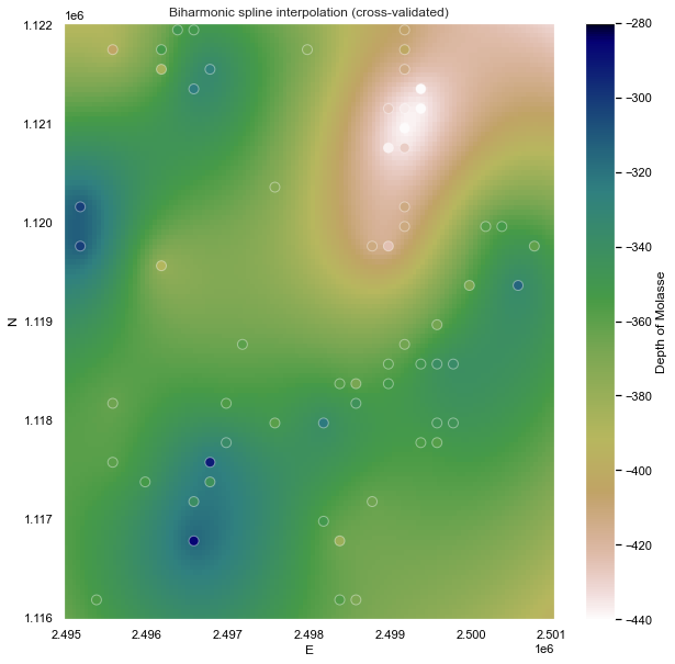
Notice that, for sparse data like these, smoother models tend to be better predictors. This is a sign that you should probably not trust many of the short wavelength features that we get from the defaults.

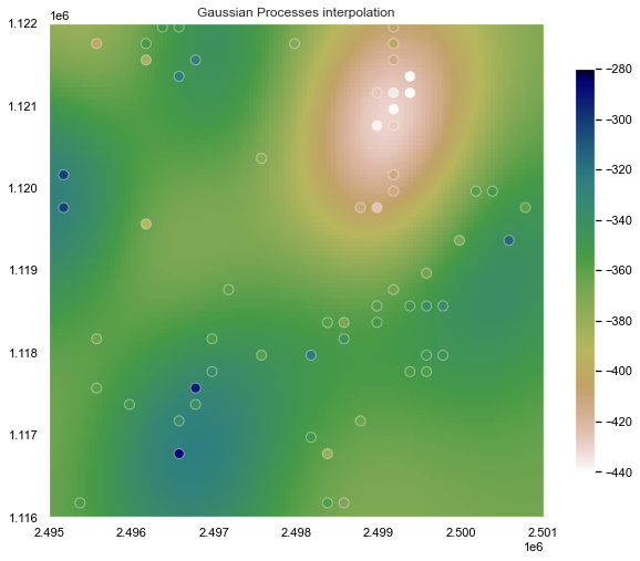
Gaussian Processes

Gaussian Processes (GP) are a generic supervised learning method designed to solve regression and probabilistic classification problems.

The advantages of Gaussian processes are:

• The prediction interpolates the observations (at least for regular kernels).
• The prediction is probabilistic (Gaussian) so that one can compute empirical confidence intervals and decide based on those if one should refit (online fitting, adaptive fitting) the prediction in some region of interest.
• Versatile: different kernels can be specified. Common kernels are provided, but it is also possible to specify custom kernels.

from sklearn.gaussian_process.kernels import RBF
from sklearn.gaussian_process import GaussianProcessRegressor as GPR
from sklearn.gaussian_process.kernels import RBF, ConstantKernel as C

kernel = C(50.0) * RBF([50 ,50])


gp = GPR(normalize_y=True, alpha=0.5, kernel=kernel,)

gp.fit(df[['E', 'N']].values, df.MOLASSE.values)

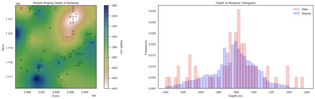
Kriging

Kriging is a widly used spatial interpolator. Here we use the [GeostatPy][https://github.com/GeostatsGuy/GeostatsPy) package (Pyrcz et al., 2021)², which is the python version of translated to Python from the original FORTRAN GSLIB: Geostatistical Library methods (Deutsch and Journel, 1997)³. Here are some important properties of kriging (Pyrcz, 2021):

• Exact interpolator - kriging estimates with the data values at the data locations
• Kriging variance can be calculated before getting the sample information, as the kriging estimation variance is not dependent on the values of the data nor the kriging estimate, i.e. the kriging estimator is homoscedastic.
• Spatial context - kriging takes into account, furthermore to the statements on spatial continuity, closeness and redundancy we can state that kriging accounts for the configuration of the data and structural continuity of the variable being estimated.
• Scale - kriging may be generalized to account for the support volume of the data and estimate. We will cover this later.
• Multivariate - kriging may be generalized to account for multiple secondary data in the spatial estimate with the cokriging system. We will cover this later.
• Smoothing effect of kriging can be forecast. We will use this to build stochastic simulations later.

The step to obtain a kriging estimate are a little more complex, first a variogram should be computed. For an in depth review of variogram calculation and modeling look here and here.

Sequential Gaussian Simulation

The objective of SGS is to building spatial models that honor the univariate and spatial distribution of the property of interest. As for Kriging some excellent resources for SGS can be found here, here, and here.

For this tutorials 10 likely realization have been generated

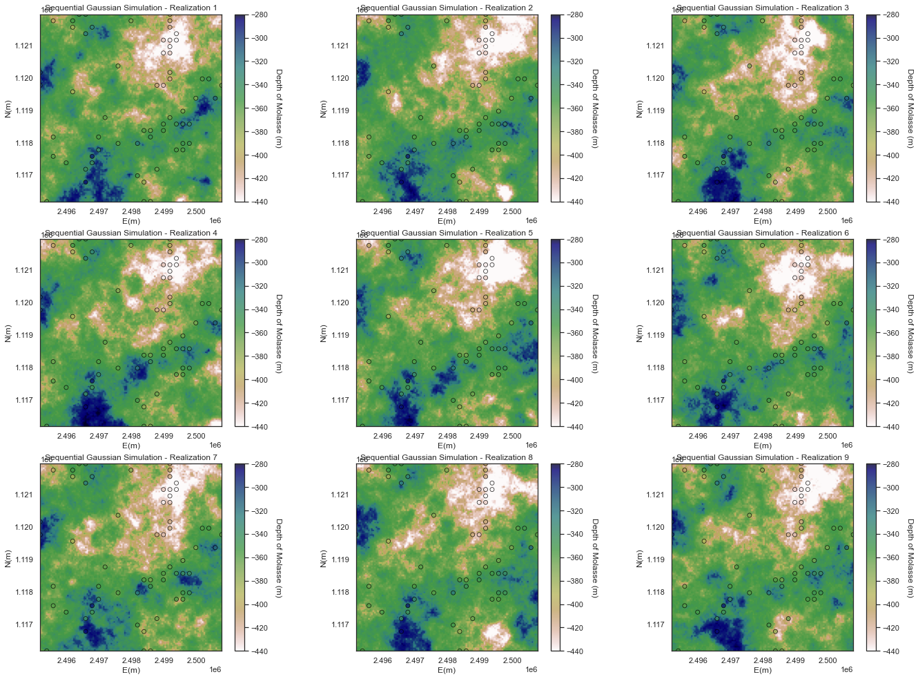
One advantage of the geostatistical simulations over Kriging and determinist interpolators is the possibility to summarize uncertainty over the realizations that is useful for:

• Quantifying local uncertainty away from wells
• Accessing the probability / risk of specific local outcomes

In particular we focus on the following local summaries:

• e-type is the local expectation (since equal weighted the same as the average)

• conditional standard deviation is the local standard deviation over the realizations

• local percentile is the local percentile over the realizations

E-type and Conditional Variance

We will start with the e-type and the conditional variance.

• e-type is the local expectation (just the average of the $L$ realizations at location $\bf{u}_{\alpha}$ as we assume all realizations are equally likely).
• conditional variance is the local variance

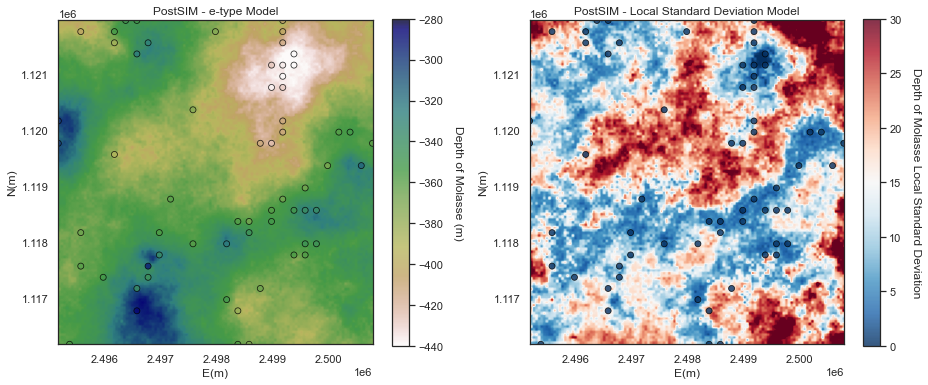
The e-type model is very similar to a kriging model, except for:

• the Gaussian forward and back transform may change the results
• result are noisy due to too few realizations

The conditional variance is lowest at the data locations and increased away from the data

• the result is noisy due to too few realizations

Local Percentiles

Now let's look at the:

• local percentile maps are the maps with the local percentile values sampled from the local realizations

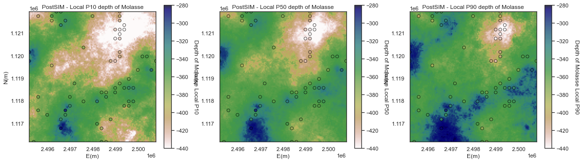
We can interpret them as follows, at a location if we have a local P10 of -300m, then we have a 90% probability of the depth is closer to the surface.

🚀🚀 Let's explore all the interpolated surfaces interactively in 3D through this app (Be patient, it takes a few seconds to wake app the Heroku dynos). 🚀🚀

That's it, enjoy interpolating with your own data! If you found this tutorial useful, please leave a comment below. 👇👇👇

Additional resources

There is a GitHub repository associated with this tutorial if you are interested.

There are lots of tutorials and resources on Dash, here is a short list of them:

Data analytics

• Youtube channel of GeostatGuy lectures
• Github of GeostatGuy with a lot, really a lot of high level resources in data analytics, geostatistics and Machine Learning
• Fatiando a Terra - Fatiando provides Python libraries for data processing, modeling, and inversion across the Geosciences

Web app

• Youtube channel of Charming Data
• Dash Bootstrap Components examples
• A journey into Plotly Dash
• Dash community forum

Python packages

[1]: Uieda, L. (2018). Verde: Processing and gridding spatial data using Green's functions. Journal of Open Source Software, 3(29), 957. doi:10.21105/joss.00957

[2]: Pyrcz, M.J., Jo. H., Kupenko, A., Liu, W., Gigliotti, A.E., Salomaki, T., and Santos, J., 2021, GeostatsPy Python Package, PyPI, Python Package Index

[3]: Deutsch, Clayton V., and A. G. Journel. 1998. GSLIB: geostatistical software library and user’s guide. New York: Oxford University Press.